Using Grover’s Algorithm to Optimize Space Design#
Quantum computing unlocks the ability to evaluate every possible state of a design, offering a glimpse into the future of how we solve complex spatial problems. By leveraging the unique properties of quantum systems, we can explore vast design spaces and isolate configurations that meet precise criteria. In this post, we will delve into Grover’s algorithm—a powerful quantum tool—and show how it enables architects and designers to reimagine spatial optimization. Just as we did in the prior posts, we’ll use Python and Cirq to demonstrate these principles in action.
What is Grover’s Algorithm?#
Grover’s algorithm is designed to tackle search problems with unprecedented efficiency compared to classical methods. At its core, the algorithm leverages quantum mechanics to explore exponentially large possibility spaces. It works by using quantum interference as we discussed in the prior post to enhance the likelihood of solutions that meet specific criteria, effectively “amplifying the probability” of their measurement while suppressing others. This process adjusts the quantum state to focus computational power on the most relevant solutions. This elegant method unfolds in two key steps:
- Oracle: Identifies and “marks” solution states by flipping their phase.(remember the how the phase can influence the amplitude in the prior post)
- Diffusion: Amplifies the probabilities of these marked states.
In classical terms, think of Grover’s algorithm as a way to search a large database where the entries meeting your criteria are tagged for easy identification. In a quantum setting, the algorithm efficiently handles exponentially large possibility spaces, making it ideal for problems like spatial optimization. This is relavant to design problems because while we might not be conducting a serach in a traditional sense, we are still trying to find the best solution to a problem. When we encode our design space as a set of qubits, we are essentially creating a database of all possible solutions. The oracle is then a function that can identify the solutions that meet our criteria.
Setting Up the Problem#
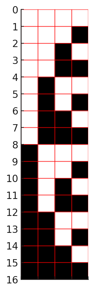
Let’s say we’re arranging four rooms in a building. Each room can be either a public or private space. Our goal is to identify layouts where either the two leftmost or two rightmost rooms are public. To achieve this, we will create a layout of qubits to represent the rooms and encode our design constraints in a quantum circuit. Specifically, we want to use an oracle function (to be explained later) to enforce the constraint that either the two leftmost or two rightmost rooms are public. Here’s how we represent this problem in a quantum circuit:
- Room Qubits (q0, q1, q2, q3): Represent the state of each room (“0” for private, “1” for public).
- Oracle Qubit (val): Flipped to indicate when a solution is found.
- Ancilla Qubits (a_adj0, a_adj1, a_xor): Store intermediate results to assist in verifying adjacency conditions.
In this example, we have four cubits allocated for all the rooms. If you think about this combinatorially, there are 2^4 = 16 possible configurations of the rooms. This is a small number, but imagine if we had 100 rooms, or if we had more complex design constraints. The number of possible configurations would be 2^100, which is an astronomically large number.
Here you can see a diagram of all the possible layouts assuming these four rooms are always arranged in a row.
Again I want to emphasize that this is a simple example, but the same principles can be applied to much more complex problems. Imagine applying this same methodology to shape grammars or other procedural algorithms that produce large populations of designs.
What are Ancilla Qubits?#
Ancilla qubits are auxiliary qubits used for temporary storage or assisting in computations. They are initialized in the |0⟩ state and reset to |0⟩ after use, ensuring no residual interference in the circuit.
Qubit Layout:#
q0, q1, q2, q3, val = qubits[:5]  # Main computation and oracle qubits
a_adj0, a_adj1, a_xor = qubits[5:8]  # Ancilla qubits for intermediate results

# a_adj0: Indicates if q0 and q1 are both public (|1⟩ state)
# a_adj1: Indicates if q2 and q3 are both public (|1⟩ state)
# a_xor: Helps check if exactly one adjacent pair is public
Constructing the Oracle#
The oracle is a crucial component of Grover’s algorithm that identifies room configurations meeting specific criteria. You can think about this as a function that allows you to “mark” the configurations that meet the design criteria. In this example, the goal is to find arrangements where only one side of the building has two adjacent rooms designated as public spaces. As we set up this algorithm, we will leverage quantum gates and ancillary qubits to encode the adjacency condition into the circuit. This is quite complex. If it’s your first time encountering this material, please consult the Quantum Gates Reference Guide for more background. Let’s break down this quantum circuit step by step, the comments will help you understand the logic:
Code for Oracle:#
q0, q1, q2, q3, val = qubits[:5]
a_adj0, a_adj1, a_xor = qubits[5:8]

# adj0 and adj1 are ancilla qubits that are used to check if the rooms are adjacent

# Example: Initial state |q0, q1, q2, q3, a_adj0, a_adj1, a_xor, val⟩ = |0, 1, 0, 1, 0, 0, 0, 0⟩

# Check if (q0, q1) are both public and if so, flip a_adj0 to |1⟩
# Example: If q0 = 1 and q1 = 1, then a_adj0 flips to 1
circuit.append(cirq.X(a_adj0).controlled_by(q0, q1))

# Check if (q2, q3) are both public and if so, flip a_adj1 to |1⟩
# Example: If q2 = 1 and q3 = 1, then a_adj1 flips to 1
circuit.append(cirq.X(a_adj1).controlled_by(q2, q3))

# Compute XOR of a_adj0 and a_adj1 to check if exactly one adjacency was found
# Example: If a_adj0 = 1 and a_adj1 = 0, then a_xor flips to 1
circuit.append(cirq.CNOT(a_adj0, a_xor))
circuit.append(cirq.CNOT(a_adj1, a_xor))

# Flip val if exactly one adjacency was found
# Example: If a_xor = 1, then val flips to 1
circuit.append(cirq.X(val).controlled_by(a_xor))

# Uncompute ancillas
# Example: Reset a_xor, a_adj0, and a_adj1 to 0
circuit.append(cirq.CNOT(a_adj1, a_xor))
circuit.append(cirq.CNOT(a_adj0, a_xor))
circuit.append(cirq.X(a_adj1).controlled_by(q2, q3))
circuit.append(cirq.X(a_adj0).controlled_by(q0, q1))
The oracle ensures that only configurations meeting the adjacency condition are marked. This process works as follows:
Check Adjacent Rooms: The oracle first checks if specific pairs of rooms (q0, q1 and q2, q3) are both designated as public (|1⟩ state). This is achieved by using controlled X gates, where the ancilla qubits (a_adj0 and a_adj1) are flipped to |1⟩ if their corresponding pair of room qubits are both in the public state.
Compute XOR: Next, the oracle calculates the XOR (exclusive OR) of a_adj0 and a_adj1 using CNOT gates. This operation helps determine if exactly one of the adjacent pairs satisfies the condition of being public, as required by the design criteria.
Mark Valid Configurations: If the XOR result is |1⟩, indicating exactly one valid adjacent pair, the oracle flips the oracle qubit (val) using a controlled X gate.
Uncompute Ancillas: Finally, the circuit reverses the operations on the ancilla qubits to return them to their initial |0⟩ state. This step ensures that the oracle doesn’t interfere with the overall computation and maintains the integrity of the quantum state.
By following these steps, the oracle tags only the configurations that satisfy the adjacency condition, paving the way for Grover’s algorithm to amplify these states effectively.
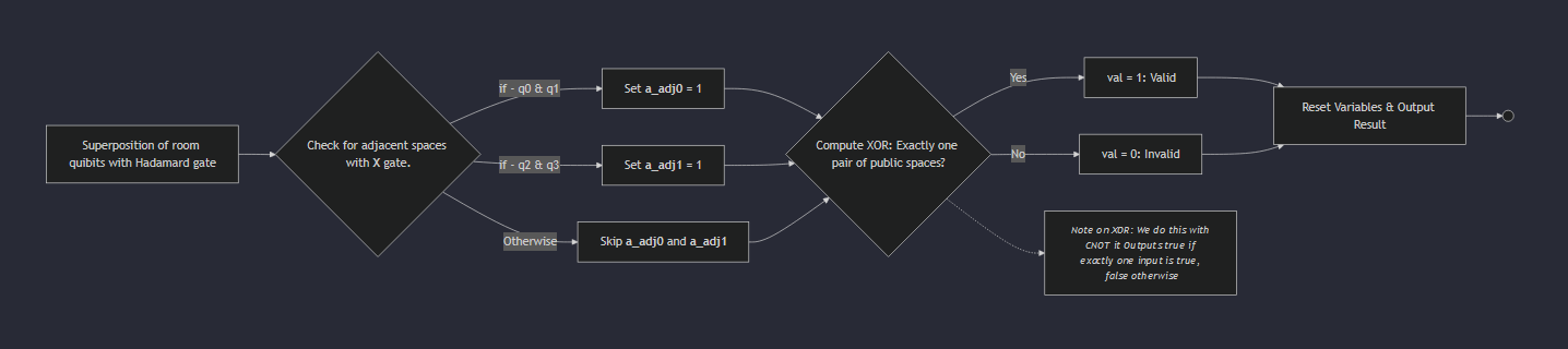
This is a diagram that maps out the oracle function.
Grover’s Algorithm Circuit#
Now, let’s tie it all together by constructing the Grover circuit:
Steps in Grover’s Algorithm:#
- Initialize Superposition: Use Hadamard gates to create an equal probability of all states.
- Oracle: Mark the solution states. (see above)
- Diffusion Operator: Amplify the probability of the marked states.
- Measurement: Collapse the quantum state to observe the result.
Code for Grover’s Circuit:#
# Step 1: Initialize superposition
circuit.append(cirq.H.on_each(q0, q1, q2, q3))

# Step 2: Grover iterations
for _ in range(num_iterations):
    # Oracle
    oracle_nonoverlapping_adjacency(circuit, qubits)

    # Diffusion
    circuit.append(cirq.H.on_each(q0, q1, q2, q3))
    circuit.append(cirq.X.on_each(q0, q1, q2, q3))
    circuit.append(cirq.H(q3).controlled_by(q0, q1, q2))
    circuit.append(cirq.X.on_each(q0, q1, q2, q3))
    circuit.append(cirq.H.on_each(q0, q1, q2, q3))

# Step 3: Measure results
circuit.append(cirq.measure(q0, q1, q2, q3, key='result'))
Diffusion Operator:#
The diffusion operator is a critical step in Grover’s algorithm. Its purpose is to amplify the probability of marked states (those identified by the oracle) while reducing the likelihood of unmarked states. This is achieved through a sequence of quantum operations that reflect the amplitudes of the states about their average value, effectively increasing the prominence of marked solutions. To understand this, we need to delve into the concepts of quantum phase and quantum state:
Quantum State: In quantum computing, a state is a vector in a complex vector space, representing the probabilities of a qubit being in the |0⟩ or |1⟩ state. A qubit can be in a superposition, meaning it simultaneously holds probabilities for both |0⟩ and |1⟩.
Quantum Phase: The phase of a quantum state is a complex number that affects the interference patterns when quantum states are combined. Phases are crucial in quantum algorithms as they can constructively or destructively interfere, altering the probability amplitudes of states.
The diffusion operator in Grover’s algorithm amplifies the probability of the marked state as follows: Marked states will have an inverted amplitude:
- First Hadamard Gates: Bring the system back into the uniform basis.
- X Gates: Prepare the reflection about |0⟩.
- Controlled-Hadamard (Diffusion Reflection): Reflects the states around the average amplitude, amplifying the marked state’s probability.
- Undo X Gates: Restore the qubits to their original basis.
- Final Hadamard Gates: Complete the reflection, resulting in amplified amplitudes for the marked state and suppressed amplitudes for all others.
This is a difficult concept to grasp, so here is a diagram that shows the reflection of the states around the average amplitude.
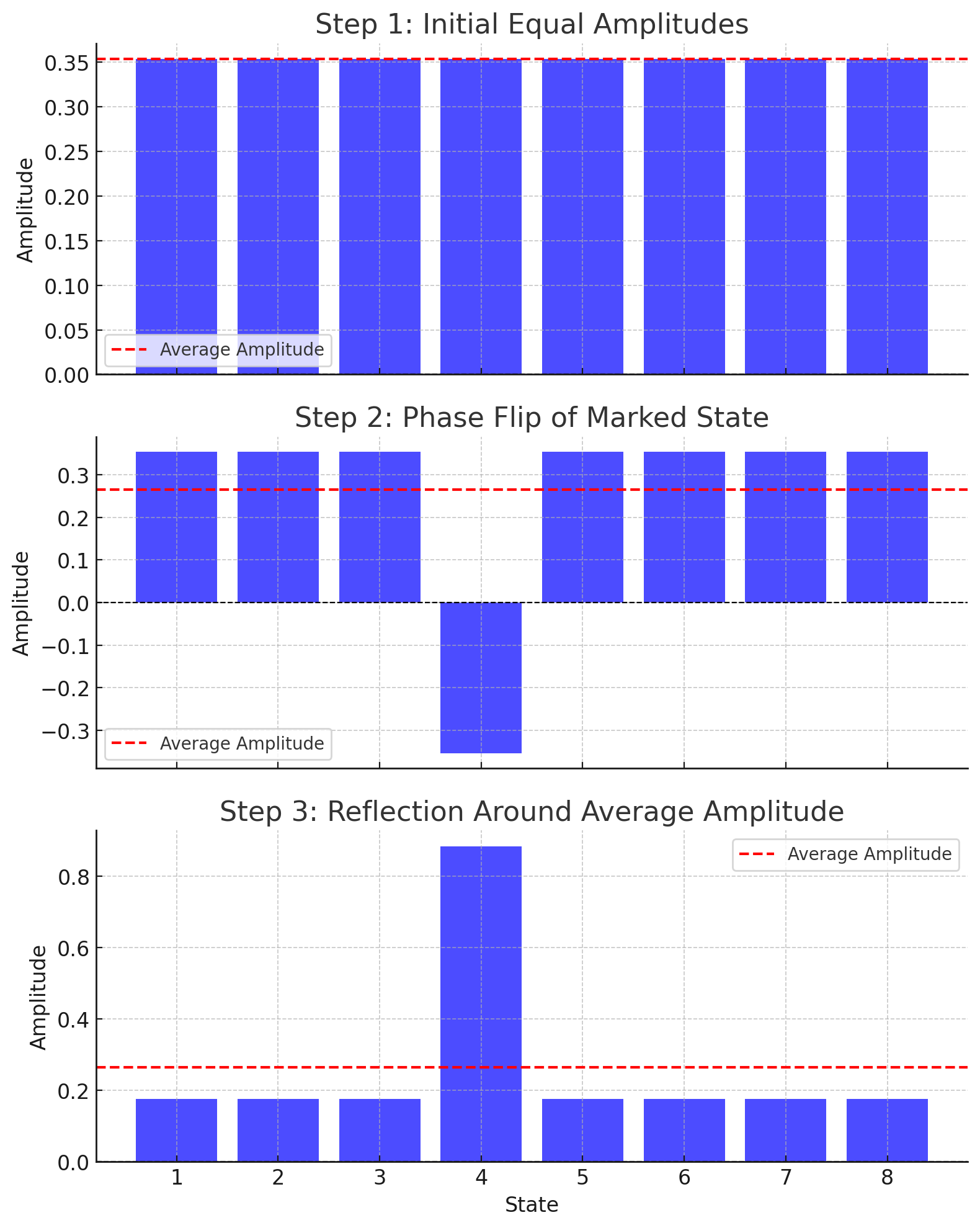
This process is performed iteratively to amplify the probability of the marked state.
Conclusion#
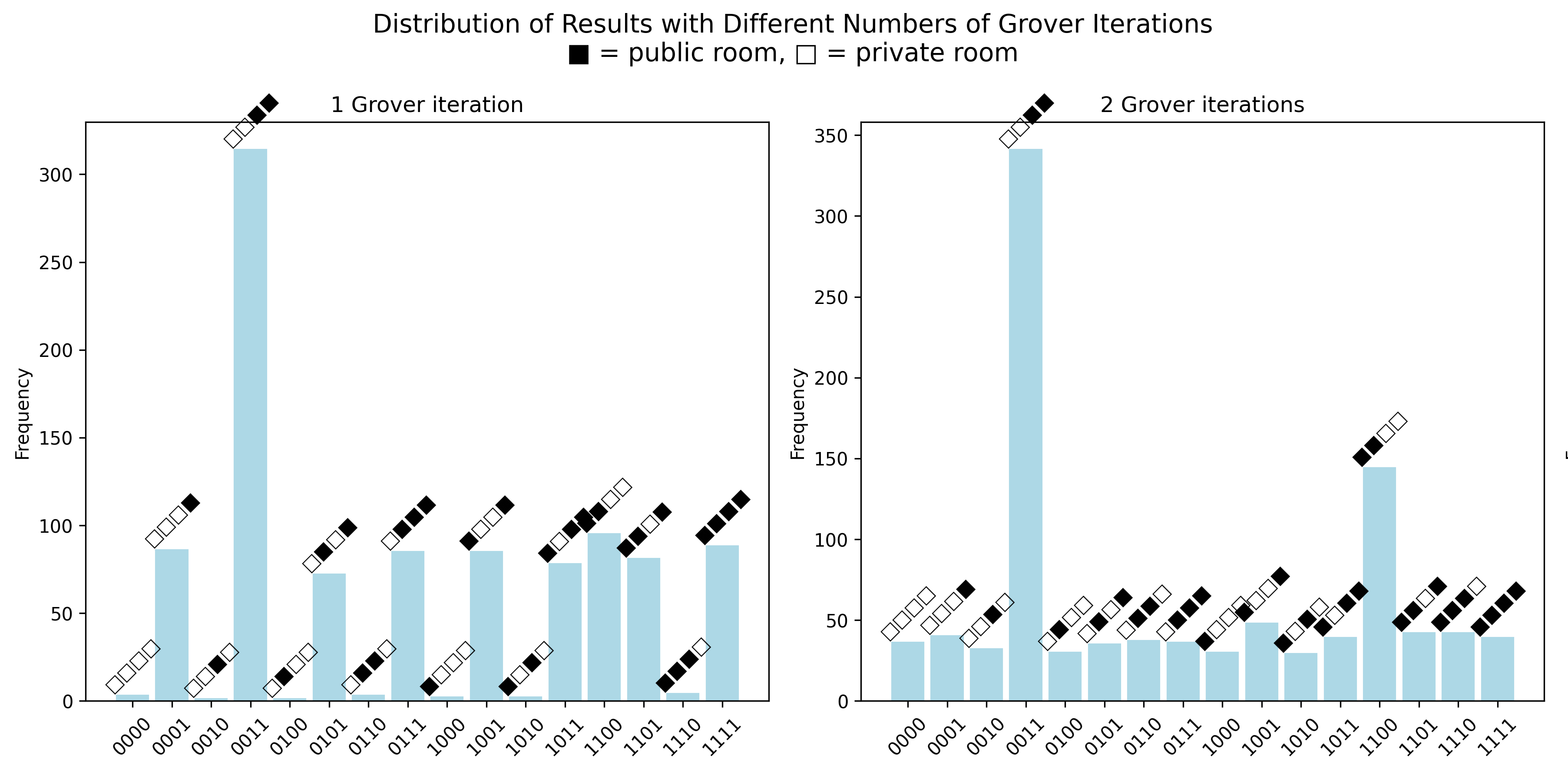
Lets take a look at the results of the circuit.
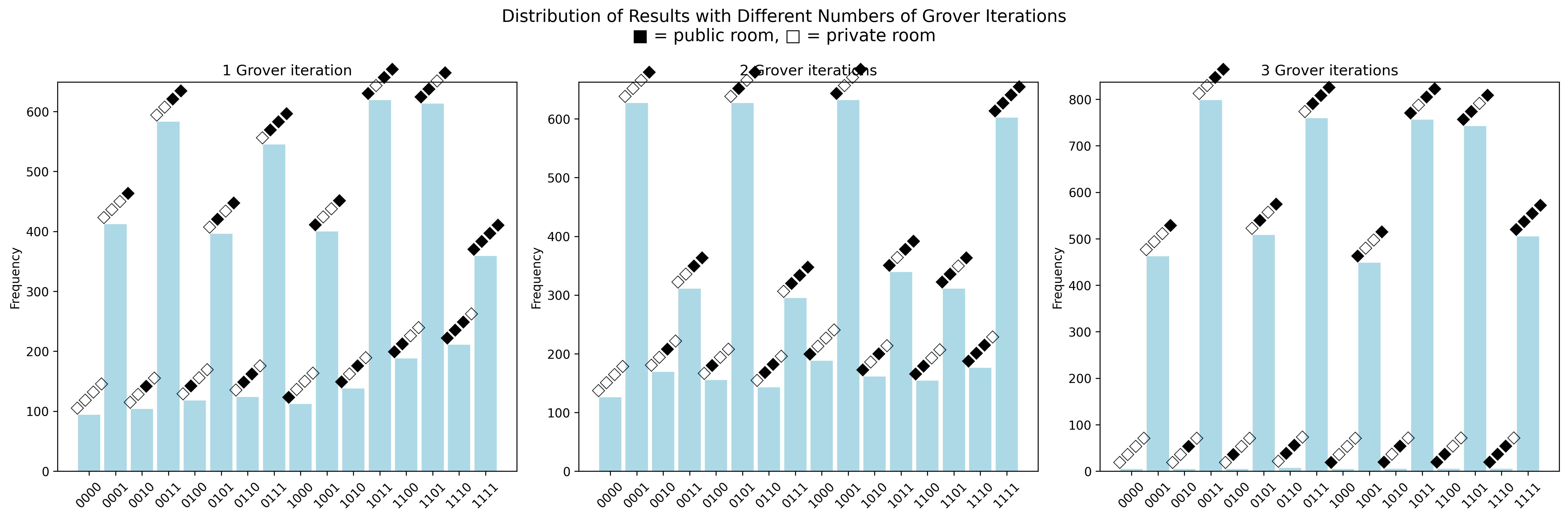
You can see the code for this example here.
This plot shows the results of the circuit. We can see that the algorithm has mostly “boosted” the probability of the configurations that meet the criteria, but there are still some configurations that are not being amplified. This is because the oracle is not perfect and there are some configurations that are not being marked, in this example 1100. This is because he oracle marks six solutions, causing the amplitude boost to be shared across a larger set of states. This often leads to weaker peaks for individual solutions and, due to quantum interference, uneven rankings. Additionally, Grover’s algorithm has an oscillatory nature—if the number of iterations isn’t tuned to the number of solutions, amplitude can constructively or destructively interfere, further influencing measurement probabilities. This highlights the tradeoff between complexity and precision when designing oracles for quantum search.
In the following image, we add some additional design constraints to the problem and limit the number of solutions to two. In this version of the algorithm the solution can only have two public spaces. As you can see, the algorithm is able to find the two solutions that meet the criteria after two iterations, highlighting how Grover’s algorithm performs better when we can tightly constrain the solution space and define the target criteria precisely.
You can see the code for this example here.
In this post, we’ve explored how Grover’s algorithm enables quantum computing to evaluate vast design spaces and isolate configurations meeting specific criteria. This approach showcases the power of quantum systems to tackle spatial optimization problems with elegance and efficiency. Imagine applying this same methodology to much harder challenges—like designing city layouts with constraints on traffic flow, resource allocation, or energy efficiency. Quantum computing provides a glimpse into a future where we can solve problems that are computationally prohibitive today, opening the door to revolutionary advancements in design and optimization.